In this post, I will be sharing my experience evaluating columnar databases against rownar databases we are all familiar with. After explaining their differences in my own words, I will answer the question: just how much faster are columnar databases are for analytics and aggregation than traditional row-based databases?
Background
To start, lets understand SQLite, the mostly commonly used single-file SQL database, stores the data for a single record is together in a contiguous block. This makes it a “rownar” file, as rows are stored sequentially. PostgreSQL adds a database management system process that manages concurrent reads and writes from other processes, but the underlying structure of how data is stored does not change.
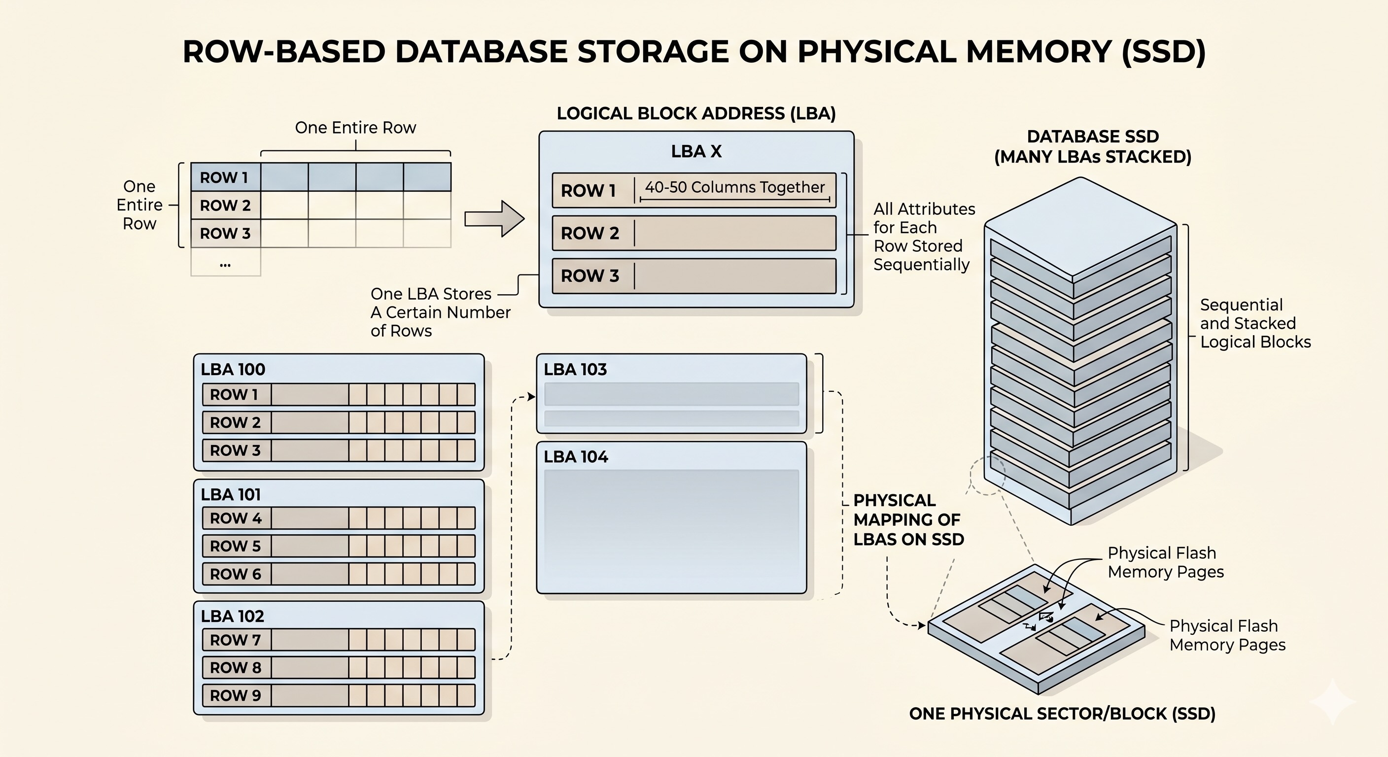
In other words, traditional row-based SQL databases store data exactly like a CSV file would. Each Logical Addressable Block (LBA) on disk stores a certain number of rows, but for each row or record, it stores every single attribute or column. This structure is excellent for OLTP, which are transactional workloads, where the access pattern often involves finding and updating only specific records using the ID, and less aggregation.
Columnar databases on the other hand, store each column or attribute in seperate LBAs. This allows each LBA to hold one attribute for every single record or entry in the database table. All values in each column are stored in ways resembling vectors, where the values are column-contiguous instead of row-contiguous. This arrangement provides optimisations in both access times and storage space. Firstly, for OLAP workloads like dashboarding, where many records from a few attributes are required.
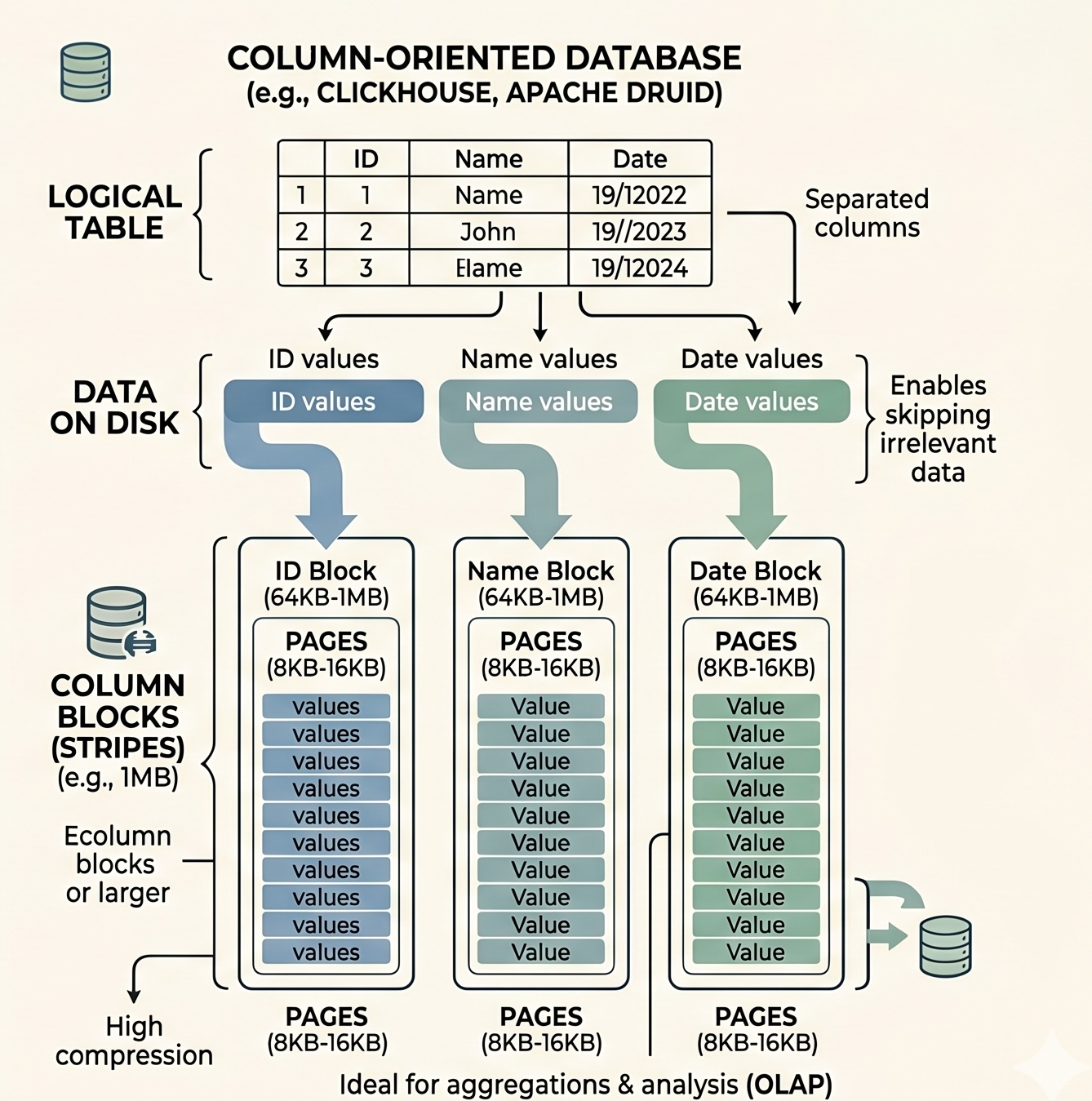
Instead of scanning through all the rows and loading all the attributes into memory before discarding those you don’t want, columnar databases only scan through the LBAs that contain data for the attributes you request, then combining them together, saving on access times and working memory requirements. Columnar database also don’t store the primary key or ID in every LBA block, instead relying on Implicit Ordinal Position, essentially keeping track of the “offset” of each entry from the starting entry, similar to an array. In terms of storage space optimisations, for attributes that contains many repeating values of the same time, like enums, compression can even further reduce the storage size.
So when to use which? Look at your access pattern. If the access pattern is more transactional when you are only updating certain entries and rarely performing row-scans, then row-based databases is the correct choice.
However, for analytical access patterns, where you retrieve large amounts of data from a few columns and performing aggregation functions like COUNT, SUM, AVG, to find insights, go with columnar databases.
The question is just how much faster are they?
Approach
For this, I simulated a typical trading ledger of a trading firm, with millions of transactions, and inserted the same data into both row-based and column-based databases. Further elaboration of the data can be found below. For the row database, I chose PostgreSQL and for the column-based database, Clickhouse is used.
Next I ran the same analytics and aggregation queries on both databases and compared the performance.
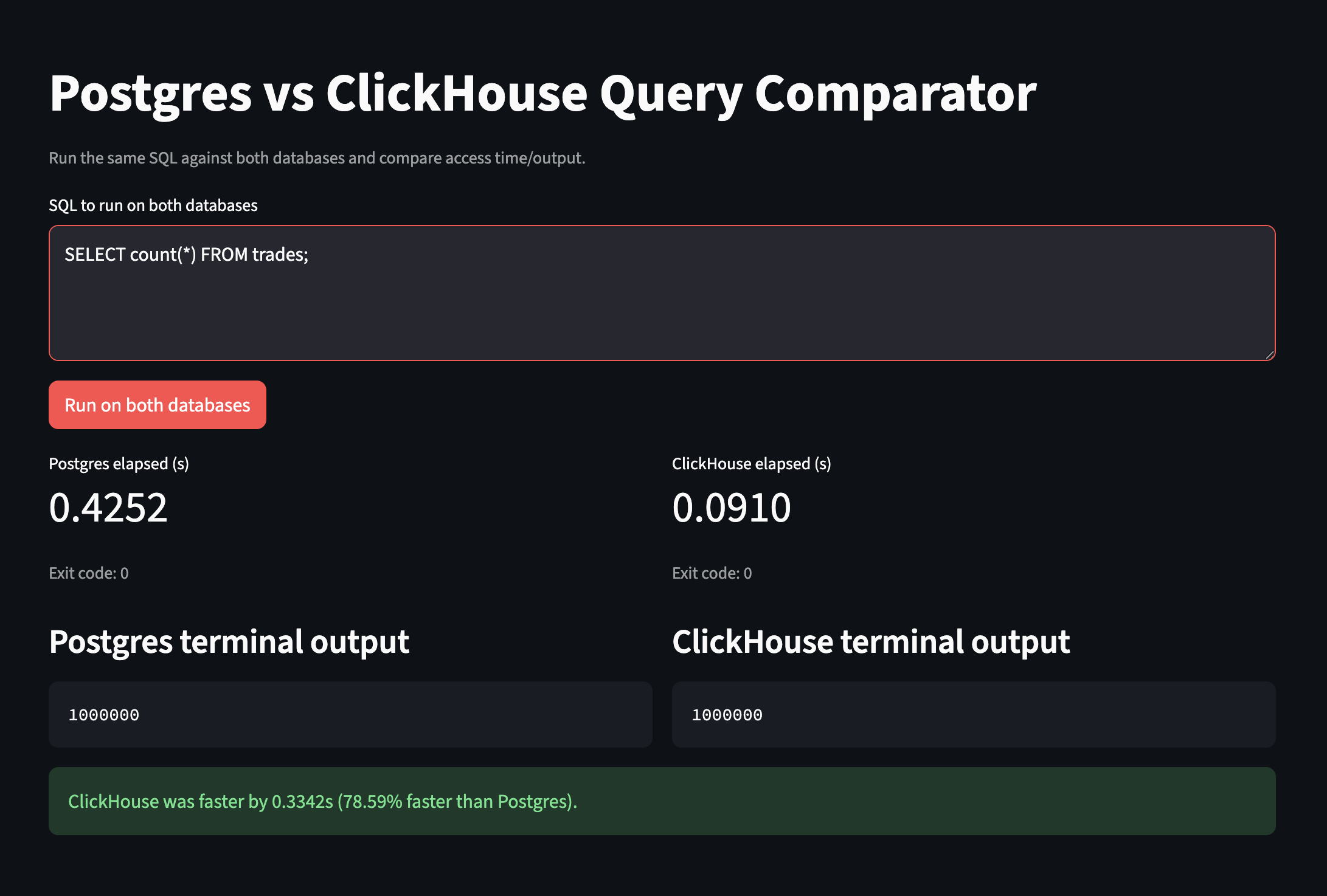
For an easier UI, I vibe-coded a streamlit dashboard which feeds the same SQL query to both Postgres and Clickhouse processes, running on seperate Docker containers on a 2024 M4 Pro MacBook Pro with 48GB of memory. The access times are displayed side by side
The dataset
5 million transactions simulating trading activity at a typical trading firm. Each transaction represents a trade executed by a specific trader, at a specific trading desk and adoption of a specific trading strategy. The full list of metadata attributes associated with each trade was suggested by Claude after brainstorming. The script for generating the dataset also takes into account other factors like bid-ask spread, latency as well as trading patterns modeled after a Pareto distribution. Note that full understanding of the meaning of each of these attributes is not crucial in the understanding of the experiment.
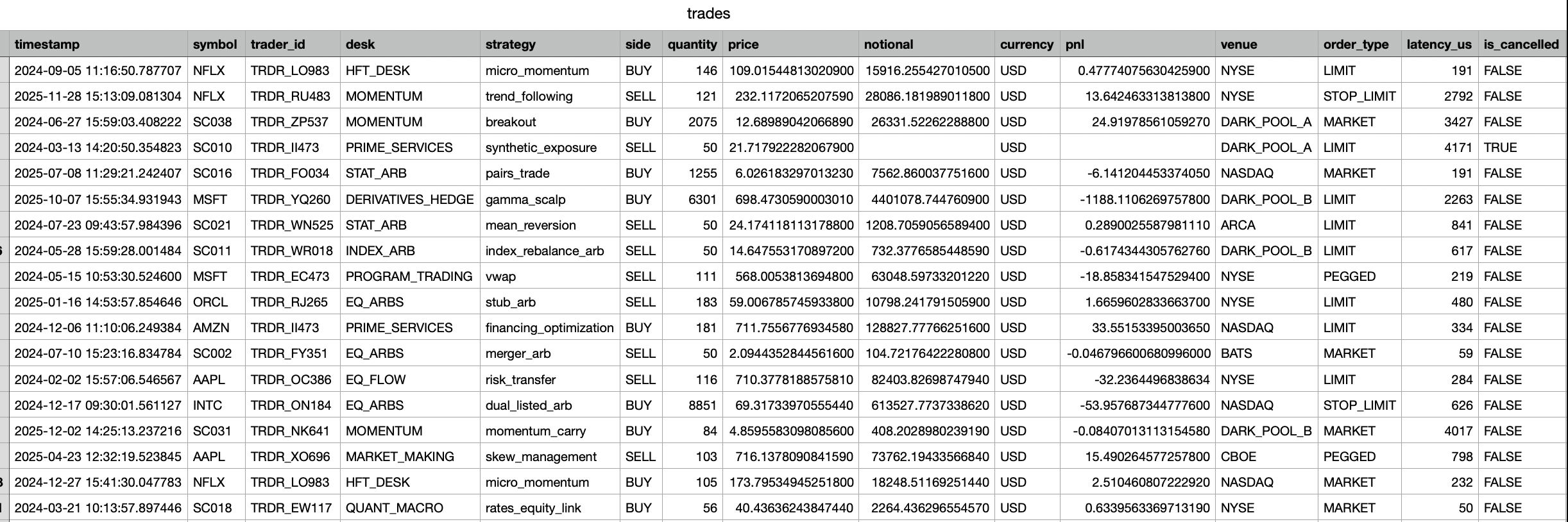
trade_idtimestamp: Generated with U-shaped intraday trading pattern, mapped to 09:30-16:00 eastern time.symbol: Basket of 80 symbols, sampled from Zipf distribution.trader_id: Trader identifier modeled after lognormal activity-weighted probabilities.desk: EQ_FLOW, EQ_ARBS, STAT_ARB, MOMENTUM, MARKET_MAKING, INDEX_ARB, RISK_ARB, QUANT_MACRO, HFT_DESK, PRIME_SERVICES, PROGRAM_TRADING, DERIVATIVES_HEDG.strategy: 70% trader-preferred strategy, 30% chance random desk-specific strategy. For full list of strategies see below.side: BUY/SELL.quantity: Based on truncated Pareto distribution sizes.price: GBM mid-price +/- half spread; spread sampled uniformly.notional: Quantity X price.currencypnl: In USD.venue: NYSE, NASDAQ, DOWJ, HKEX, SGX.order_type: MARKET, LIMIT, PEGGEDlatency_us: Order-type baseline uniform latency + venue delays. HKEX highest latency.is_cancelled: Probability modelled by Bernoulli outcome by order type and desk.counterparty_id
Strategy enums (strategy) by desk: I have no idea what they are
- EQ_FLOW: client_facilitation, risk_transfer
- EQ_ARBS: merger_arb, dual_listed_arb, stub_arb
- STAT_ARB: pairs_trade, mean_reversion, cointegration
- MOMENTUM: trend_following, breakout, momentum_carry
- MARKET_MAKING: passive_quote, skew_management
- INDEX_ARB: index_rebalance_arb, etf_nav_arb, basis_trade
- RISK_ARB: event_driven, capital_structure_arb, vol_arb
- QUANT_MACRO: cross_asset_rotation, macro_factor, rates_equity_link
- HFT_DESK: latency_arb, queue_fade, micro_momentum
- PRIME_SERVICES: financing_optimization, synthetic_exposure, inventory_rotation
- PROGRAM_TRADING: basket_execution, vwap, twap, is_algo
- DERIVATIVES_HEDGE: delta_hedge, gamma_scalp, vega_rebalance
Queries used for 5 million entries
- Simple sanity check. Selecting the first 1000 rows.
SELECT * FROM trades LIMIT 1000;
- End of day aggregation of PNL by each trading desk (with its strategy)
SELECT
    CAST(timestamp AS DATE)          AS trade_date,
    desk,
    strategy,
    COUNT(*)                         AS trade_count,
    SUM(pnl)                         AS total_pnl,
    AVG(pnl)                         AS avg_pnl,
    MIN(pnl)                         AS worst_trade,
    MAX(pnl)                         AS best_trade,
    SUM(notional)                    AS total_notional
FROM trades
WHERE
    is_cancelled = FALSE
    AND pnl IS NOT NULL
    AND timestamp >= '2022-01-01'
    AND timestamp <  '2024-01-01'
GROUP BY
    CAST(timestamp AS DATE),
    desk,
    strategy
ORDER BY
    trade_date ASC,
    total_pnl DESC;
- Top 25 traders by Notional trading volume within a quarter
SELECT
    trader_id,
    desk,
    COUNT(*)                                        AS trade_count,
    SUM(notional)                                   AS total_notional,
    SUM(CASE WHEN side = 'BUY'
             THEN notional ELSE 0 END)              AS buy_notional,
    SUM(CASE WHEN side = 'SELL'
             THEN notional ELSE 0 END)              AS sell_notional,
    AVG(notional)                                   AS avg_notional_per_trade,
    SUM(pnl)                                        AS total_pnl,
    SUM(latency_us * notional) / SUM(notional)      AS notional_wtd_latency
FROM trades
WHERE
    is_cancelled = FALSE
    AND notional IS NOT NULL
    AND timestamp >= '2023-01-01'
    AND timestamp <  '2023-04-01'
GROUP BY
    trader_id,
    desk
ORDER BY
    total_notional DESC
LIMIT 25;
- Cartesian product of Symbol × Desk × Currency
SELECT
    symbol,
    desk,
    currency,
    side,
    COUNT(*)                                            AS trade_count,
    SUM(CASE WHEN is_cancelled = TRUE
             THEN 1 ELSE 0 END)                         AS cancelled_count,
    SUM(notional)                                       AS total_notional,
    AVG(price)                                          AS avg_price,
    STDDEV(price)                                       AS price_stddev,
    SUM(pnl)                                            AS total_pnl,
    AVG(pnl)                                            AS avg_pnl,
    AVG(CASE WHEN pnl > 0
             THEN 1.0 ELSE 0.0 END)                     AS win_rate,
    AVG(latency_us)                                     AS avg_latency_us,
    MAX(notional)                                       AS max_notional
FROM trades
WHERE
    timestamp >= '2022-01-01'
    AND timestamp <  '2024-01-01'
GROUP BY
    symbol,
    desk,
    currency,
    side
ORDER BY
    total_pnl DESC;
The results
Query 1:
This is a simple scan of n number of entries, selecting all attributes.
For less number of rows like 100, postgres egdes clickhouse out by 3.50% But for as the number of rows increase, their access times converge at around 1100 rows. At 5000 rows, Clickhouse was 27.59% faster than Postgres.
Query 2:
This involves reading 4 attributes: desk, strategy, notional value and PNL from a specific date range. In this case it is a day. Postgres would perform a full sequential scan, reading all columns, while ClickHouse reads only 4 column files and performs a vectorised SUM.
Surprisingly, Postgres was actually faster by 0.0049s (6.05% faster than ClickHouse).
One reason could be that the number of entries within the date range might be too little for the advantages of columnar database to take effect. While Postgres does have to load all columns, Clickhouse on the other hand, has to read from 4 seperate blocks to find the 4 columns. For a small number of entries, the overhead from accessing seperate 4 LBA blocks might outweigh the savings, especially if only a small number of entries are read from each block. In this case, Postgres is able to scan through the small number of entries quicker. If the date range was larger say one month, we could expect Clickhouse to be faster.
Query 3:
This is query is similar to the previous, requiring a scan over a date range but only requesting for a few attributes: trader_id, desk, notional value and PNL
Result: Clickhouse beat Postgres by 25.82%
This is case is exactly what we expected from the previous query! Since this query involves entries over a quarter instead of only a day, there are way more entries so the speed of access for each attribute that Clickhouse provides far outweigh the overhead from opening multiple blocks. Even with a B-Tree based index on the timestamp column in Postgres, the penalty from full row loads from disk was enough to slow it down significantly.
Query 4:
This cartesian product is one of the most expensive aggregation queries for row-based databases like Postgres. The cross-product of three dimensions, each with large number of unique values(cardinality) creates a large number of groups, requiring alot of data to be held in memory.
Result: Clickhouse yields a 56.02% advantage over Postgres!
Although time complexity O(m x n x p) is the same, Postgres's hash aggregate operates row-by-row, while ClickHouse's hash aggregation uses Single Instruction Multiple Data (SMID) vectorisation on each column, meaning it operates on the whole column at once, this makes combining data for cross products extremely efficient. At 80 symbols × 12 desks × 5 currencies = up to 4,800 groups, and 5M entries, the difference in memory access patterns is quite significant.
Conclusion
Columnar databases offers many clever optimizations for working with analytical or aggregation based workloads, where it really shines when accessing just a few attributes from a table with a large number of rows. Techniques like vectorized operations and compression also offer performance and storage savings.
Other interesting takeaways learnt from this project's research
- Zipf law, which describes the phenomenon of heavyweight over representation. Formally, the probability of the k-th ranked item is proportional to 1/k^s where s is the exponent. The less common an item is, the less often it appears. This almost perfectly describes the stock market, where the first 10 most liquid symbols (Tier 1) like $NDVA, $APPL,$MSFT occupy the top ranks and collectively absorb ~60–70% of all trades. Tier 3 symbols at ranks 36–80 each appear rarely.
- U-shaped intraday timing representing a larger trading volume at start of the day and end of the day, while the middle of the has lower trading volume.
- The Pareto distribution (also called a power-law distribution) describes phenomena where a small number of events account for most of the “mass.” Interesting this also perfectly describes number of trades against trade quantities, where there are a very large number of small quantity trades (retail investors) followed by a very long tail of a few enormous trade quantities (institutional investors)
- Geometric Brownian Motion (GBM) is used for modeling randomness mid market prices,thereby helping these trading firms determine their bid-ask spreads for daily and intraday price changes.
Future learnings:
- Learn about the different types of trading strategies
- Bernoulli models for side and cancellation outcomes.
Check out the repo here.